The Functional Style Part 8: Persistent data structures.

We have discussed immutability at length by now. In particular, we have covered how loops can be replaced with recursive function calls to do iteration while avoiding reassignment of any variables. While it might seem on the face of it that this technique would be grossly inefficient in terms of memory, we have seen how tail call elimination can negate the need for extra subroutine calls, thus avoiding growing the call stack, and making functional algorithms essentially identical to their imperative equivalents at the machine level.

So much for scalar values, but what about complex data structures like arrays and dictionaries? In functional languages they are immutable too. Therefore, if we have a list in Clojure:

(def a-list (list 1 2 3))

and we construct a new list by adding an element to it:

(def another-list (cons 0 a-list))

then we now have two lists, one equal to (1 2 3) and the other (0 1 2 3). Does this mean that, in order to modify a data structure in the functional style, we have to make a whole copy of the original, in order to preserve it unchanged? That would seem grossly inefficient.

However, there are ways of making data structures appear to be modifiable while preserving the original intact for any parts of the program that still hold references to it. Such data structures are said to be ‘persistent’, in contrast with ‘ephemeral’ data structures, which are mutable. Data structures are fully persistent when every version of the structure can be modified, which is the type we will discuss here. Structures are partially persistent when only the most recent version can be modified.

Fully stacked.

The stack is a very good example for how to implement a persistent data structure, because it also shows a side benefit of this technique. The code happens to get simpler too; we will come to that in a moment.

Because we are creating a functional stack here, our interface looks like this:

public interface Stack<T> {

    Stack<T> pop();

    Optional<T> top();

    Stack<T> push(T top);
}

Given that this is a persistent data structure, we can’t ever modify it, so on pushing or popping we get a new Stack instance that reflects our pushed or popped stack. Any parts of the program that are holding references to previous states of the stack will continue to see that state unchanged.

For obtaining a brand new stack, we will provide a static factory method:

public interface Stack<T> {
    
    ... // pop, top, push
    
    static <T> Stack<T> create() {
        return new EmptyStack<T>();
    }
}

It might seem a strange design choice to create a specific implementation for an empty stack, but when we do it works out very tidily. This is the benefit I mentioned earlier:

public class EmptyStack<T> implements Stack<T> {

    @Override
    public Stack<T> pop() {
        throw new IllegalStateException();
    }

    @Override
    public Optional<T> top() {
        return Optional.empty();
    }

    @Override
    public Stack<T> push(T top) {
        return new NonEmptyStack<>(top, this);
    }
}

As you can see, top returns empty and pop throws an illegal state exception. I think it is reasonable to throw an exception in this case, because given the last in first out nature of stacks and their typical uses, any attempt to pop an empty stack indicates a probable bug in the program rather than a user error.

As for the non-empty implementation, that looks like this:

public class NonEmptyStack<T> implements Stack<T> {

    private final T top;
    private final Stack<T> popped;

    public NonEmptyStack(T top, Stack<T> popped) {
        this.top = top;
        this.popped = popped;
    }

    @Override
    public Stack<T> pop() {
        return popped;
    }

    @Override
    public Optional<T> top() {
        return Optional.of(top);
    }

    @Override
    public Stack<T> push(T top) {
        return new NonEmptyStack<>(top, this);
    }
}

It’s worth noting that choosing separate implementations for the empty and non-empty cases avoided the need for any conditional logic. There are no if statements in the above code.

In use, the stack behaves like this:

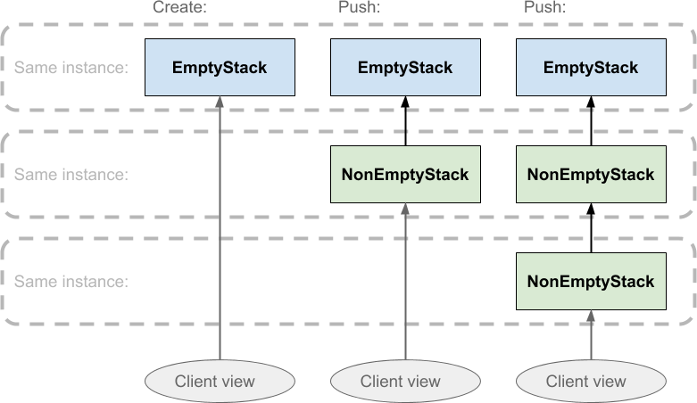
1. Stack.create returns an EmptyStack instance.
2. Pushing on it returns a NonEmptyStack with the pushed value as its top.
3. When another value is pushed on top of the non-empty stack, another NonEmptyStack instance is created with the newly pushed value on top:

The timeline here runs from left to right, and the ovals at the bottom of the diagram represent the ‘view’ the client sees of the stack. The regions bounded by dashed lines indicate that all the boxes within are all the same object instance. The direction of the arrows show that each NonEmptyStack instance holds a reference to another stack instance, its parent, which will either be empty or non-empty. This parent object reference is what will be returned when the stack is popped, and that is where things get clever:

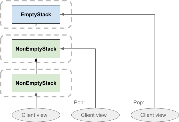
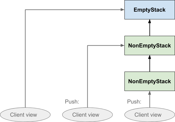
On popping the stack, the client simply shifts its view to the previously pushed element. Nothing gets deleted. This means that, if there were two clients with a view of the same stack, one client could pop it without affecting the other client’s view of the stack. The same is true of pushing:

This is basically the same as the first diagram, except that we have dispensed with the horizontal dashed regions and instead made it explicit that the stack is a single data structure rather than several copies. We are simply representing each Stack instance, whether empty or not, as a single box. Initially the client sees an empty stack; on pushing, a non-empty stack instance is created which points at the empty stack, and the client shifts its view to the new instance. When the client pushes a second time, another non-empty stack instance is created which points at the previous non-empty stack, and the client shifts its view again. The stack tells the client where to point its view next, via the return value of the push and pop operations, but it is the client that actually shifts its view. The stack does not move anything.

Now you might be thinking that "the client shifts its view" implies something is being mutated, and indeed it does, but this is simply a variable holding a reference to a Stack instance. We have discussed at length already in part 2 of the series how to manage changing scalar values without having to reassign variables.

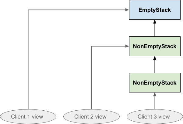
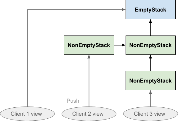
We already mentioned the possibility that different parts of the program might be holding separate and different views on the stack structure, so now let’s explicitly imagine that the three ovals represent three different clients’ views of one single stack structure. Client 1 is looking at a newly created stack, client 2 has pushed once on it, and client 3 has pushed twice on it:

If client 2 subsequently pushed something on the stack, the effect would look like this:

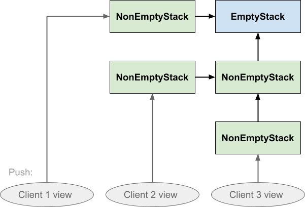
Notice the directions of the arrows ensure that neither client 1 or client 3 are affected by what client 2 did: client 3 cannot follow the arrow backwards to see the value that was just pushed, and nor can client 1. Similarly if client 1 pushed on the stack neither of the others would be affected by that either:

The other thing to note about this data structure is that nothing is duplicated. All three clients share the same EmptyStack instance, and clients 2 and 3 also share the NonEmptyStack that was pushed first. Everything that could be shared is shared. Nothing is copied whenever any of them push, and popping does not cause any links in the structure to be broken.

So when do things get deleted? Eventually we must reclaim resources or our program may run out of memory. If a stack element has been popped, and no part of the program is holding a reference to it any more, in time it will be reclaimed by the garbage collector. Indeed, garbage collection is an essential feature for functional programming in any language.

Cons cells, CAR and CDR.

This stack structure might seem familiar to you. If it does, it's for good reason. This structure is known as a linked list and it is a foundational data structure in computer science. Usually linked lists are represented by a diagram something like this:

The list is a chain of elements, and each element contains a pair of pointers. One of the two pointers points to a value. The other one points at the next element in the chain, except for the final element in the chain which does not point to another element. In this way a chain of values can be linked together. One advantage usually cited for this kind of data structure, in imperative programming, is that it is very cheap to insert a value in the middle of a list: all you need to do is create the new element, link it to the following element, and re-point the preceding element in the list to the new element. The elements of a linked list do not have to be contiguous in memory, nor do they need to be stored in order, unlike an array. An array would require shuffling all the elements down after the inserted element in order to make room for it, which could be a very expensive operation indeed. On the other hand, linked lists perform poorly for random access, which is an O(n) operation. This is because to find the nth element you must traverse the preceding (n - 1) elements, unlike an array where you can access any element in constant O(1) time.

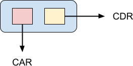
Linked lists are an essential data structure in functional programming. The Lisp programming language is literally built out of them. In Lisp, a single element of a linked list is referred to as a cons cell:

The CAR pointer points to the value of the cons cell while the CDR pointer points to the next element in the list. CAR and CDR are archaic terms which are not in general use any more, but I mention them for historical interest, and perhaps you might come across them. The Lisp programming language was first implemented on an IBM 704 mainframe, and the implementers found it convenient to store a cons cell in a machine word. The pointer to the cell value was stored in the “address” part of the word, while the pointer to the next cell was stored in the “decrement” part. It was convenient because the machine had instructions that could be used to access both of these values directly, when the cell was loaded into a register. Hence, contents of the address part of the register and contents of the decrement part of the register or CAR and CDR for short.

This nomenclature made it into the language; Lisp used car as the keyword for returning the first element of a list, and cdr for returning the rest of the list. Nowadays, Clojure uses first and rest for these instead, which is much more transparent: it is hardly appropriate to name fundamental language operations after the architecture of a computer from the 1950s. Other languages might refer to them as head and tail instead.

The creation of a new cons cell is referred to as cons-ing and it therefore means to create a list by prepending an element at the beginning of another list:

user => (cons 0 (list 1 2 3))
(0 1 2 3)

Just as we saw in the stack example, cons-ing an element onto a list does not alter the list for any other part of the program that is still using it.

Binary trees.

That’s all fine, but what about if we want to insert a value in a list, or append it to the end? In this case duplication is necessary; we will have to duplicate all the elements up to the point in the list where the new element is to be inserted. In the worst case - appending an element to the end - we will be forced to duplicate the entire list.

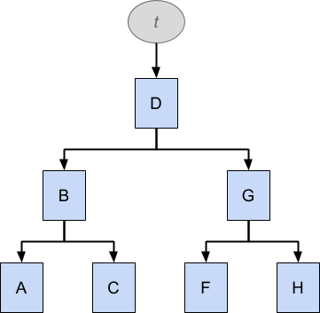
Another approach is to use a binary tree instead of a linked list. This is an ordered data structure in which every element has zero, one or two pointers to other elements in the structure: one points to an element whose value is considered lower than the current element, and the other points to an element whose value is considered greater, by whatever comparison is appropriate for the type of data held in the tree:

A binary tree can be searched considerably more efficiently than a linked list, but it needs to be balanced for optimum performance. To be optimal, the top element of the tree must be the median of all the values in the tree, and the same must be true for the top elements of all the sub-trees as well. In the worst case, when a binary tree becomes completely skewed down either side, it becomes indistinguishable from a linked list.

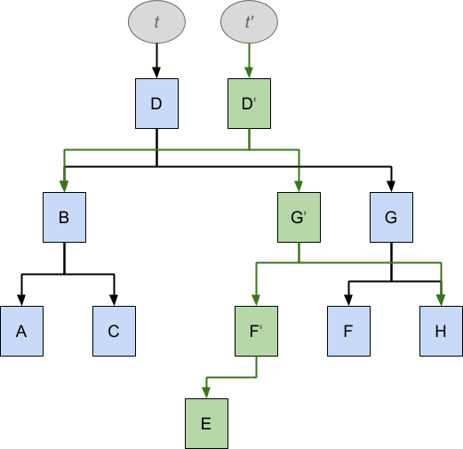
The structure t above holds a tree of elements that are ordered alphabetically: A, B, C, D, F, G, H. Notice that E is missing. Following the arrows down, elements to the left have lower value than elements to the right, so you can easily traverse the tree to find a value by comparing the value with each element in turn and following the tree down+left or down+right accordingly. Such data structures are therefore good for searching, and a generalised variant called a B-tree is commonly used for indexing database tables.

Now let us imagine that we want to insert the missing value E into this tree, which might look in code like this:

t' = t.insert(E)

As before, we want this insertion operation to leave the original tree t unmodified, while at the same time we would like to reuse as much of t as possible in order to minimise duplication. The result looks like this:

To achieve the insertion of E it has been necessary to duplicate D, G, F, while A, B, C are shared between the two data structures, but the effect is that, following the arrows from t the original data structure is unchanged, while following the arrows from t' we see a data structure that now also includes E in the proper position.

One direction.

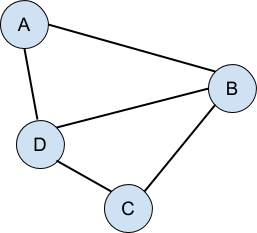
The linked list and the binary tree have one vital thing in common: both are examples of directed acyclic graphs. If you haven’t heard this term before, don’t be dismayed, because it’s very simple. A graph is a collection of things (nodes, points, vertices, whatever) that have connections between them:

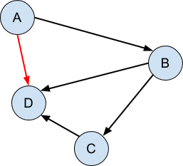
The graph is directed when the connections only go one way:

Finally, the graph is acyclic when there are no cycles, that is to say, it is impossible to follow the graph from any point and return back at that same point:

It is the directed acyclic nature of these structures - that the connections can be followed in one direction only and never loop back on themselves - that make it possible for us to ‘bolt on’ additional structure to give the appearance of modification or copying, while leaving unaffected any parts of the program that are still looking at the original version of the structure.

Don’t panic!

I’m hoping that my explanations here have made some sense, but if not, don’t worry too much. It’s not necessary to implement data structures like these when you do functional programming - functional and hybrid-functional languages have immutable data structures built in which work just fine, very probably better than anything most of us could write.

My reason for including this section in the series is partly technical interest - I like to know how things work - and partly to allay concerns about efficiency. Immutable data structures do not mean making wholesale copies of entire structures every time something needs to be modified; much more efficient methods exist for doing this.

Next time.

This concludes our introduction to the fascinating subject of functional programming. I hope it’s been useful. In the next article, we will finish up with some final thoughts. We will discuss the declarative nature of the functional style, and whether functional and object-oriented programming styles can live together. We will briefly look at one of the benefits of functional programming that I did not really go into much in this series - ease of concurrency - and consider the tension between the functional style and efficiency concerns.

Part 1 - Introduction

Part 2 - Getting Started

Part 3 - First-Class Functions I: Lambda Functions & Map

Part 4 - First-Class Functions II: Filter, Reduce & More

Part 5 - Higher-Order Functions I: Function Composition and Monads

Part 6 - Higher-Order Functions II: Currying

Part 7 - Lazy Evaluation

Part 8 - Persistent data structures

Part 9 - Pragmatism

Follow the author on Twitter